ForgeGIS · Digital Twin · Transport

The plume that checks its own math

A conserved scalar carried on a wind while it spreads.

The ForgeGIS twin engine’s transport operator has something most simulation code never gets: a closed-form external truth. Act I holds it against the analytic Gaussian solutions and reports the errors to the decimal. Act II takes it to the coast — one hypothetical release, paused mid-event, forked five ways off a single anchor — with the divergence read off the conservation ledger. Every claim on this page is checked against the recordings.

0.0005%
Error in the simulated variance slope against the analytic law σ²(t) = σ₀² + 2Dt — on both axes
2.1e-8
Worst per-epoch mass drift over 60 epochs behind closed walls — float32 rounding, not a leak
6 worlds
One paused run, five sibling forks off a single anchor epoch, all living in one recording
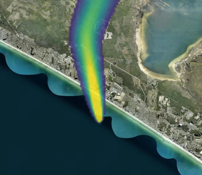
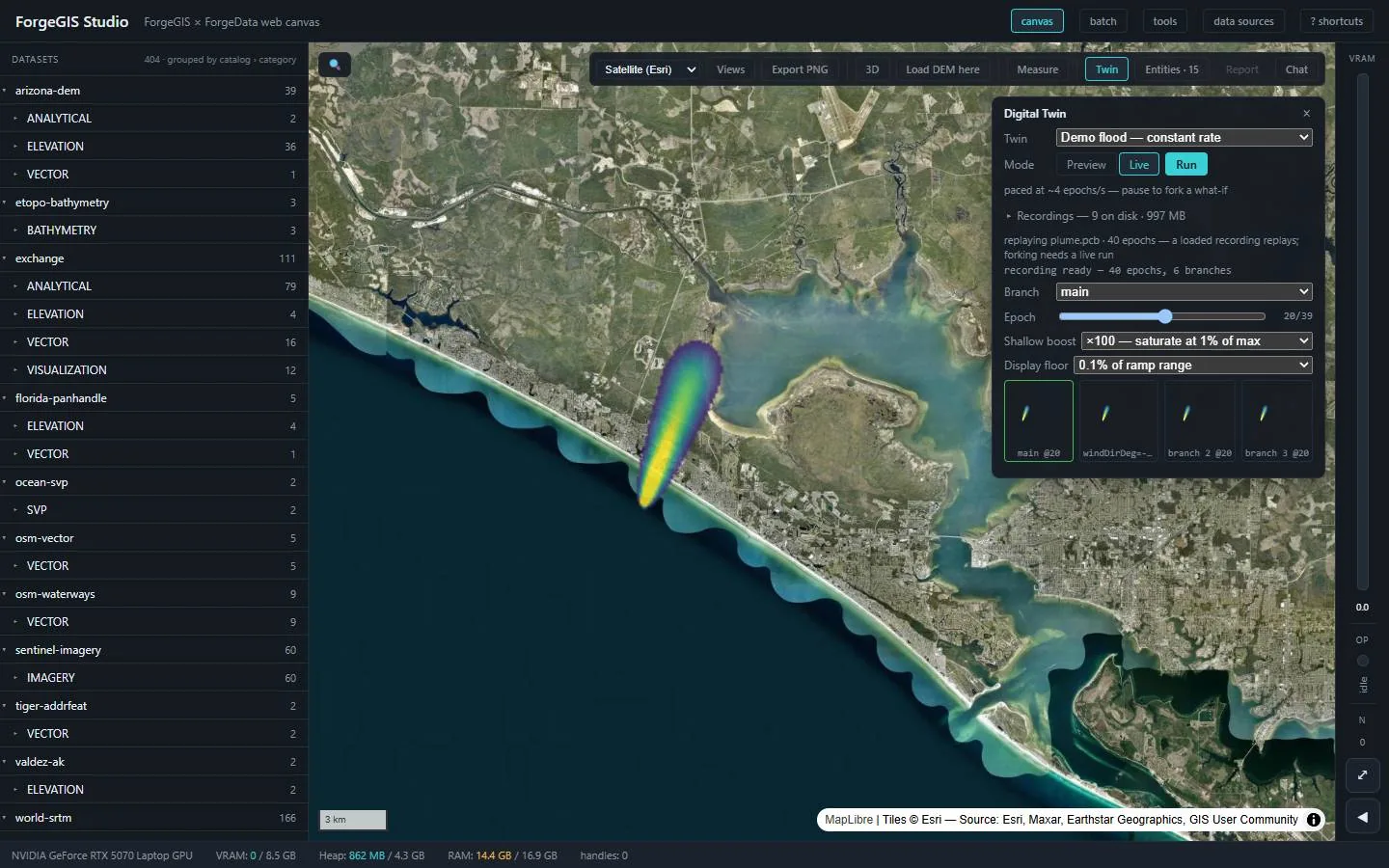
The ForgeGIS Studio browser workspace: a dataset catalog on the left, a satellite map of the Panama City Beach coastline in the centre with a compact bright plume running inland from the shore, and a Digital Twin panel at the top right showing branch main at epoch 20 of 39
The decision moment, replayed from the recording: the main branch at the fork anchor, epoch 20 of 39, about 6.8 km of plume up the 20° track from the hypothetical coastal release. The panel is holding a loaded recording — 40 epochs, 6 branches — with the branch thumbnails at the bottom showing the same cursor epoch in each world.

How to read the numbers

What the units mean, and where the model stops being literal. Worth two minutes before the charts.

The conserved quantity
A dimensionless transport quantum. The ledger counts “stuff per cell,” not µg/m³, and this page never pretends otherwise.
Distance
Grid cells. Act II’s 256² grid over a 0.30° × 0.25° box puts one cell at ≈113 m — that conversion is geometry, and it is the only physical unit on the page.
The clock
A model tick, not a calibrated second. Wind speed is cells-per-tick, with the CFL bound windSpeed·Δt/substeps ≤ 1 enforced by refusal rather than clamping. So read shapes, ratios and conservation bookkeeping — never “concentration at 3 PM.”
Scope, stated everywhere it matters: this page validates the transport engine against closed-form analytic solutions. It is not a calibrated dispersion model — no turbulence closure, no Pasquill–Gifford stability classes, no buoyancy, no deposition, no meteorological data — and it is not comparable to HPAC, HYSPLIT, or AERMOD.
Act I

The analytic validation

Three runs on a synthetic flat world — no terrain, because the operator is deliberately terrain-free in v1 — registered directly against the twin API and read back through the same endpoints the Studio panel uses: exact cell values and mass-weighted moments, never pixel luminance. The operator under test is corner-transport upwind advection plus explicit five-point diffusion, operator-split, substepped, behind closed walls.
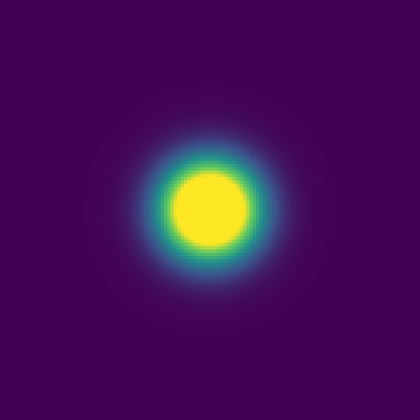
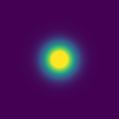
A compact bright disc of concentration with a hard-edged yellow core on a dark field
t = 2
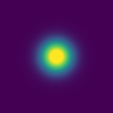
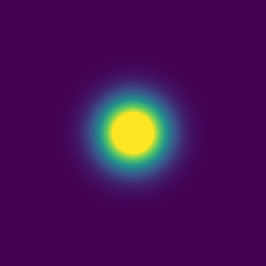
The same bump, slightly broader, its yellow core smaller and its blue-green halo wider
t = 16
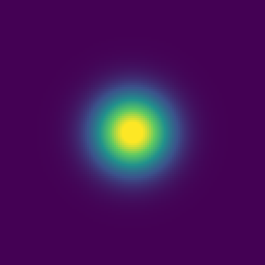
The bump broader again, the yellow core reduced and the surrounding gradient softer
t = 31
A wider, softer bump with a small dim yellow centre and a broad graded halo
t = 46
The widest and softest of the five: a broad graded bump whose yellow centre has nearly faded into the green surround
t = 60

One bump, no wind, closed walls, five sampled ticks of the same run. The core dims and the halo widens — and the total never changes. Both of those are laws with closed forms, and the run is held to both.

Simulated variance against the analytic diffusion law, sim time 0 to 60 Measured variance on both the x and y axes rises linearly from about 106 square cells at t equals 1 to about 165 at t equals 60, lying on top of the analytic law sigma-zero squared plus 2Dt with D equal to 0.5. The fitted slope is 0.999995 against an analytic 2D of 1 — 0.0005 percent off — so the three curves are drawn on top of one another and are visually indistinguishable. 0 50 100 150 200 0 15 30 45 60 measured σx² and σy² — on the line on the line analytic σ₀² + 2D·t (D = 0.5) measured σx² measured σy² sim time t (model ticks) variance (cell²)
The flagship check. Discrete five-point diffusion is exactly linear in the interior, so the variance of the bump must grow at exactly 2D per unit of sim time. The fitted slope is 0.999995 against an analytic 2D = 1 — on both axes, with no fitting in the line drawn. All three curves lie on top of one another; that is the result.
Per-axis variance grows at 2D per unit of sim time
observedslopeX 0.999995, slopeY 0.999995expected2D = 1 ± 2%
Diffusion is isotropic — the two axes agree
observed|slopeX − slopeY| = 4.08e-8expected< 1e-3 · 2D
Conservation oracle: closed walls, no source, total mass flat across all 60 epochs
observedworst per-epoch relative deviation 2.103e-8expected< 1e-5 (float32 rounding)
Determinism: raw frames of a re-run hash byte-identical at every sampled epoch
observede0 4a3658fd · e20 eee871ba · e40 9d4ec274 · e59 c365c06d — all equalexpectedsame sha256 per epoch

The second solution: a plume in a wind

A continuous source in a steady wind, run to steady state. The Gaussian plume has three signatures, and each is read off the final frame’s raw cells rather than fitted to them: column mass exactly equal to the injection (conservation), width growing linearly downwind (the width law), and the centerline falling as 1/σy — the 1/√x law.

Why this run is holdable at all

At CFL = 1 the advection pass is an exact one-cell shift, which is what lets the steady plume be held against the pure-diffusion Gaussian with no numerical-diffusion correction applied anywhere.
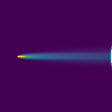
A dark field with a narrow bright streak running from a source near the left edge due east, broadening and fading downwind, with a thin bright band at the right edge of the frame
The steady plume: source near the left edge, wind due east, the cone the Gaussian predicts. The bright band at the right edge is the closed wall doing exactly what a closed wall does — mass that reaches it piles up rather than leaving.
Cross-wind sections at two downwind distances against their moment-fitted Gaussians Two measured cross-sections through the steady plume, one at 40 cells downwind peaking near 0.25 quanta per cell and one at 70 cells downwind peaking near 0.19, each plotted against a Gaussian fitted from its own moments. Measured and fitted curves overlie one another; the normalized RMS residual is 0.20 percent of peak at 40 cells and 0.10 percent at 70 cells. The section further downwind is lower and wider, which is the plume width law. 0.00 0.10 0.20 0.30 −16 −8 0 8 16 measured @ 40 cells downwind measured @ 70 cells downwind Gaussian fitted from the section’s own moments cross-wind offset from centerline (cells) concentration (quanta/cell)
Two slices across the plume, each against a Gaussian fitted from its own moments. The measured curves sit on the fitted ones to within 0.20% of peak at 40 cells and 0.10% at 70 — and the further slice is lower and wider by exactly the amount the width law requires.
Steady column mass equals the per-substep injection exactly — a conservation law, not a fit
observedcol d=40: 2.0000 · col d=70: 1.9998expected2 ± 2%
Plume width grows at the analytic rate per downwind cell (the width law)
observedΔσy² = 7.4721expected7.5 ± 10%
Centerline decays as 1/σy — the 1/√x law
observedC(40)/C(70) = 1.3245expectedσy(70)/σy(40) = 1.3201 ± 10%
The cross-sections really are Gaussian
observedNRMS 0.20% @ d=40, 0.10% @ d=70expected≤ 5% of peak
Act II

One anchor, six futures

A hypothetical release at a point on the coast — no real facility; the coordinates are a stage, not a scenario — carried inland on a 20° wind at 3 cells per tick. At epoch 20 the run pauses, and the operator’s question is the one that actually gets asked in a room: which way does the sky go, and how big is the source really? So the run forks five sibling branches off that one anchor: a wind-shift through the panel’s fork form, a three-branch wind-direction fan, and a 10× source fork through the API.

Scope, again, because it matters here most: the wind is a constant twin parameter — a what-if knob, not weather. There is no met data, no sea-breeze cycle and no boundary layer anywhere in this run, and nothing on this page is a forecast for anywhere.

Pause, then branch

The what-if form opens on the paused branch and exposes exactly what is forkable: the twin was registered with windSpeed, windDirDeg and sourceRate as declared constants, and that is precisely what makes them fork knobs. Here the wind direction is backed 30°, from 20° to −10°. Nothing else is touched.

The rule, stated on the form

The note under the fields states the contract the whole capability rests on: branches differ by parameters only; the fork anchors where this branch paused. The status line reads main: PAUSED @ epoch 20, and that is the anchor every one of the five siblings inherits.
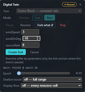
The Digital Twin panel with a Paused badge, the Fork what-if control active, fields for windSpeed set to 3, windDirDeg set to -10 and sourceRate set to 8, a Create fork button, and a status line reading main: PAUSED at epoch 20
The what-if form on a run paused at epoch 20. All three declared constants are present as editable knobs; windDirDeg is being taken from 20° to −10° for the branch.

Same epoch. Different sky.

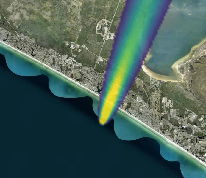
Both frames are epoch 39 in two worlds that share every byte of history to epoch 20 and nothing after it.
Baseline — wind 20°
Satellite view of the coastline with a bright plume running inland from the shore to the north-northeast, over the built-up strip and toward the bay at the upper right
Backed wind — −10°
The same satellite view at the same epoch with the plume running almost due north instead, staying west of the bay

Left, the baseline track runs inland to the north-northeast. Right, the branch after the wind backs 30°: the same source, the same history, a plume that leans almost due north and misses everything the baseline crossed. The only difference between these two frames is one number, changed once, 19 epochs earlier.

Concentration at the receptor across six worlds sharing one history to epoch 20 Six timelines share one history until epoch 20, where the run is forked. The baseline rises from zero after epoch 16 and settles near 0.17 quanta per cell. The 10x source fork follows the baseline and then climbs steeply past epoch 36 to about 0.54. The backed-wind branch and the three-branch wind fan all rise briefly and then collapse to zero — on-track winds arrive at the receptor; the backed wind never does. 0.00 0.20 0.40 0.60 0 10 20 30 40 the fork anchor · epoch 20 epoch 20 baseline — 0.17 backed wind — never arrives backed wind source 10× wind-direction fan — 320°, 50°, 80° epoch receptor concentration (quanta/cell)
The decision study: concentration at a receptor about 7 km downwind on the baseline track, in all six worlds. One line to epoch 20, then six. On-track winds arrive; the backed wind never does — 1.713e-1 against 5.694e-6 at epoch 39, a collapse of more than four orders of magnitude from one number changed once.
Total scalar mass, baseline against the 10x source fork Total scalar mass in the domain rises linearly in the baseline at 8 quanta per tick, reaching about 320 quanta by epoch 39. The 10x source fork leaves the baseline at the epoch 20 anchor and rises at 80 quanta per tick, reaching about 1688 by epoch 39. The gap between them at epoch 39 is 1368 quanta, which is exactly what the closed form predicts. 0 500 1.0k 1.5k 2.0k 0 10 20 30 40 the fork anchor · epoch 20 epoch 20 source fork — 80/tick baseline — 8/tick 1,368 quanta 1,368 epoch total scalar mass (quanta)
The same fork, quantified by the ledger instead of the picture. The branch injects at ten times the baseline rate from the anchor on, so the wedge between the two worlds is not an emergent surprise — it is a closed form. At the shared epoch 39 the ledger measures 1367.998 quanta against a predicted 1368.000. Conservation is the divergence oracle.
All three declared constants are fork knobs in the form
observedwindDirDeg + sourceRate + windSpeed fields presentexpected3 fields
Six worlds off one anchor: baseline plus five sibling forks, every one anchored at epoch 20
observed5 forks created — wind −10°, 320°, 50°, 80°, source 10×expectedwind-shift + 3-fan + 10×-rate, all siblings of timeline 0
The recording’s own rows say fan, not chain: every fork is a child of timeline 0 at the same anchor
observedt1←0@20 t2←0@20 t3←0@20 t4←0@20 t5←0@20expectedall ←0@20
The 10× wedge equals the closed form — conservation as the divergence oracle
observedmeasured 1367.998 vs closed form 1368.000 @ shared epoch 39expectedequal to 1%
The wind-shift what-if is the receptor’s whole story: the backed wind carries the plume away
observedbaseline 1.713e-1 vs backed-wind 5.694e-6 at epoch 39expectedshifted < 25% of baseline
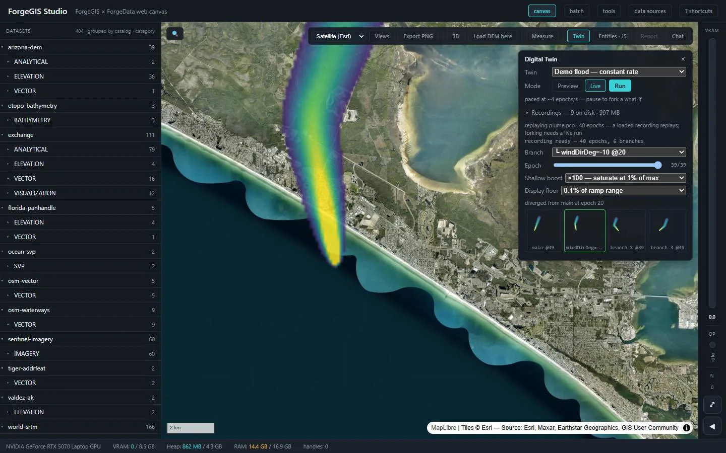
The ForgeGIS Studio workspace zoomed in on the coastline with a large plume curving inland to the north, the Digital Twin panel showing the branch selector set to windDirDeg=-10 at epoch 39 of 39 and a row of four branch thumbnails at the same epoch
The backed-wind branch on the canvas at the last epoch of the run, with the branch selector reading windDirDeg=−10 @20 and the note diverged from main at epoch 20. The thumbnail row underneath is the n-up replay: every branch rendered at the one cursor epoch, so worlds are compared at the same moment rather than from memory.

What this page is honest about

The limits are part of the result. A validation that hides its regime is not a validation.

Engine validation, not dispersion modeling

The real comparators are elsewhere

Operational plume work belongs to HPAC, HYSPLIT and AERMOD — models with turbulence closures, stability classes, source physics and decades of field calibration. This page is none of that. It demonstrates that the twin engine’s transport is exactly the equation it claims to solve — the property those models assume of their own solvers — and that the twin contract holds around it.

Uniform wind, no weather

One constant vector, whole grid

No met data, no sea-breeze cycle, no boundary layer. That is exactly what makes the wind-shift fork honest: it is a parameter study over an idealized field, not a forecast for anywhere.

Terrain-free, closed walls

The coast is a basemap, not physics

v1 transport ignores topography entirely, and the domain edge is a closed wall — mass that reaches it piles up rather than leaving. Validation runs are sized so nothing reaches a wall, and the conservation check depends on the walls being closed.

First-order scheme, disclosed regime

Where the extra spreading is, and isn’t

Corner-transport upwind is first-order: off the CFL = 1 axis it adds numerical diffusion with a known closed form. The validation runs sit where that term is exactly zero; the Act II worlds run where the extra spreading is real but small — and disclosed, not hidden.

Display settings on the screenshots are disclosed and display-only: a shallow boost, because the 10× fork’s source otherwise dominates the shared colour ramp, and a display floor at 0.1% of the ramp, because a diffusing scalar stays float32-nonzero far past anything meaningful and that underflow halo would paint as an opaque disc that reads like a footprint. The floor is a fraction of the ramp, not a threshold of concern — the ledger is untouched by either.

Want the depth behind this?

The full technical showcase carries the blocks this page condenses — definition hashes, run identifiers, every recorded API exchange, and the Java probes that pin the same cards cell-by-cell. Seaglass Foundry is happy to walk an evaluator through it.

rich@seaglassfoundry.com